Previously we examined the technical SEO data to get more precise technical recommendations that will make your website content more discoverable and meaningful to search engines using Exploratory Data Analysis (EDA). EDA is where we inspect the statistical nature of the site’s SEO features such as word count.
Single site audits don’t yield competitive insights
Technical SEO data for a single site is useful for having a scientific understanding and it gives you some empiricism to secure buy-in from your colleagues. However, it’s rather limited in that it lacks context and thus insight to glean competitive advantage.
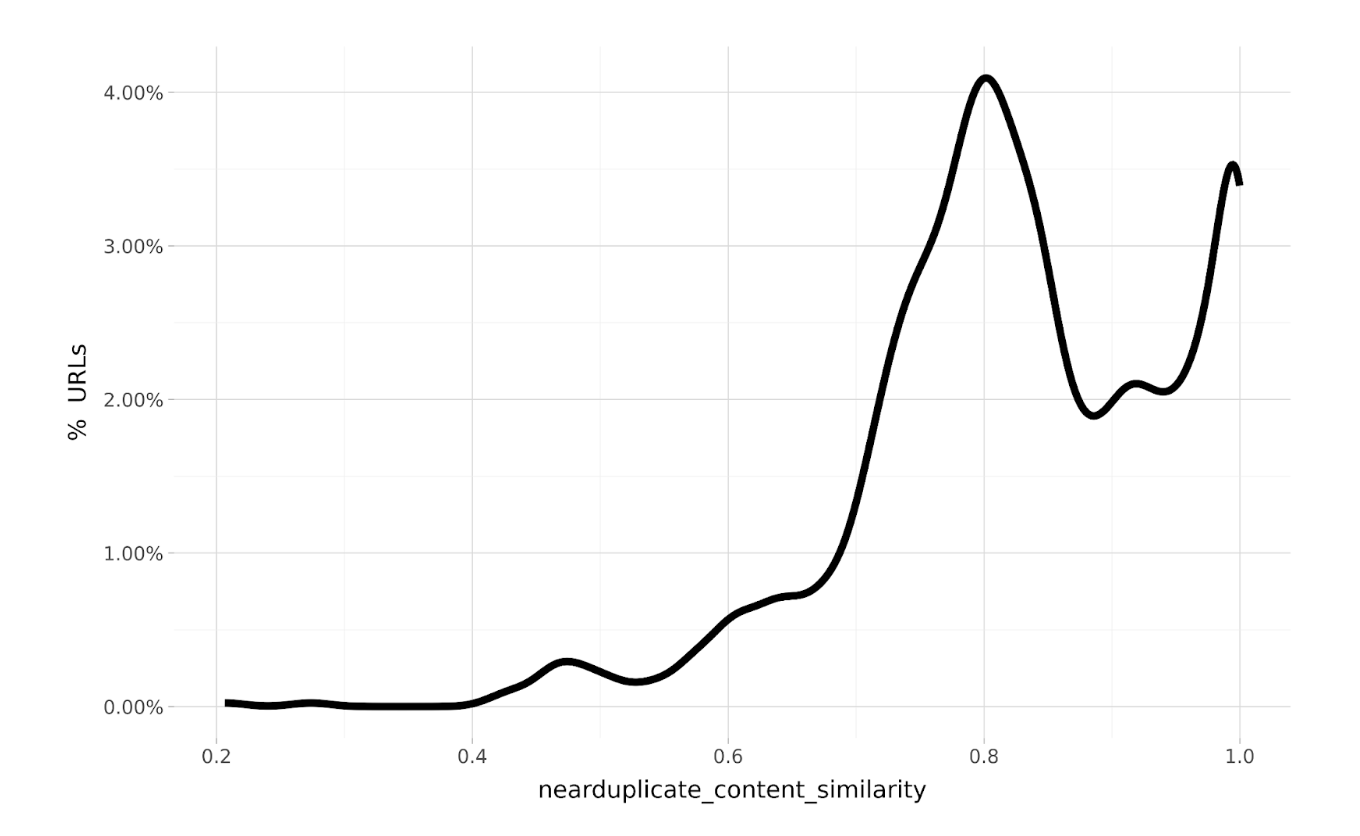
For example, take the near duplicate content metric we examined last time.

We see the average for the client is 80% – but compared to market or industry competitors – is that good? Bad? Average? Should we be worried?
Auditing your competitors
It doesn’t matter what the technical ranking factor is, we cannot begin to answer these questions without data against which to compare.
Where can we get that data? By crawling your competitors. Of course, some industries are much more competitive than others, implementing anti-crawl bot measures (even towards their own SEO teams!) – so this option may not always be possible.
However, if you can – you should at least try to crawl your competitors and get the data. Once done and exported, you can then import these with Python by combining an iterator block with the Pandas read_csv function like below:
import pandas as pd
import glob
import os
# Define the folder path containing your oncrawl CSV export files
folder_path = "path/to/your/folder"  # Change this to your actual folder path
# Get a list of all CSV files in the folder
oncrawl_csv_files = glob.glob(os.path.join(folder_path, "*.csv"))
# Read and concatenate all CSV files into a single DataFrame
oncrawl_raw_df = pd.concat((pd.read_csv(file) for file in oncrawl_csv_files), ignore_index=True)
# Display the combined DataFrame
display(oncrawl_raw_df)
Comparing distributions
Once the data is imported into your Python notebook you can start exploring each technical SEO feature – only this time with multiple websites.
That way you get to see the context of how your site compares to other websites within your competitor space.
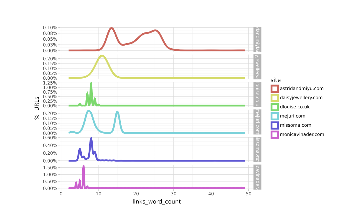
For example, the plot below compares the statistical distribution of the ratio of internal links count to body word count for a number of luxury jewelry websites.

Code to generate:
from plotnine import ggplot, aes, geom_density, facet_grid, labs
# Create the density plot faceted by 'site' (arranged by rows)
feature_plot = (
    ggplot(oncrawl_raw_df, aes(x="links_word_count", color ="links_word_count")) +
    geom_density(alpha=0.5) +
    facet_grid("site ~")  # Facet by 'site', arranged in rows
)
display(feature_plot)
Please note that while this feature is not currently part of the Oncrawl analysis, I derived it from the two features that are: word count and internal links. I did this because I had the hypothesis that search engines would suffer more internal links if there’s more textual content on the page i.e. less of a link farm.
As we can see from the chart, we get a sense of range where Monica Vinader and D Louise sites are quite consistent in their ratios, less than 10, indicating consistent template designs. The Astrid & Miyu site on the other hand is least consistent with ratios from 10 to 30.
In terms of skew, all sites, to varying degrees, are positively skewed where most of the data sits on the left i.e. mostly lower values and outliers have higher values.
With the exception of the Daisy London Jewellery site, most sites are multi-modal when it comes to the links to word count ratio i.e. multiple most frequent values shown by multiple peaks. This is highly indicative of different content design templates which exhibit similar behaviors and thus the values congregate around these template types e.g. product categories (Product Listing Pages PLPs) and items (Product Detail Pages PDPs).
[Ebook] Data SEO: The Next Big Adventure
The different peaks vary for each site with Monica Vinader site having the lowest ratio of internal links per word count to the Astrid & Miyu site with the most. That’s usually a good sign as that variation is likely to explain the variation in performance.
While we don’t know the direction of performance i.e. is a higher ratio of internal links per word count better or worse for performance? Now, we have a clue.
Regression analysis
Regression analysis solves the problem of understanding the performance direction of variation by comparing the values with performance.
Naturally, your clients competitors are unlikely to willingly disclose their performance analytics data to help your client, so third party SEO traffic data sources using URL as the primary key will help you do the trick using the Pandas merge function, something like:
import pandas as pd

# Perform a left merge on the "url" column
regression_df = oncrawl_raw_df.merge(seo_analytics_df, on="url", how="left")

# Display the first few rows of the merged DataFrame
display(regression_df)
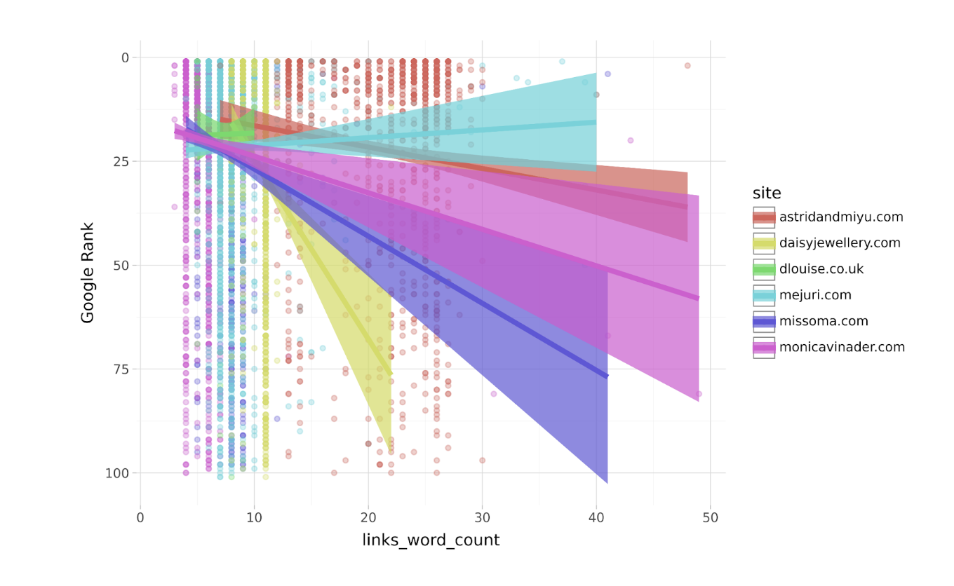
In the case of the chart below, we continue with the ratio of internal links to word count example:

We see that in the case of luxury jewelry in the UK search space, it’s beneficial to have less internal links per word count.
This may be quite obvious to the more experienced SEO readers among you; however, having the data to visualise and support your recommendations will make your professional life much easier.
While it’s increasingly fashionable to bash rank positions as an SEO performance metric, it still works surprisingly well for gaining competitive insight advantages. And even in the era of AI search, you still need to nail the basics of technical SEO.
You may even surprise yourself with the insights revealed to you by cycling through the features offered by Oncrawl.
Quantifying the performance benefit of technical features
Of course, rather than plotting and viewing two charts for every feature, machine learning can make quick work of this by modeling the data to quantify how much rank benefit each technical SEO feature offers.
The model process works by:
- Cleaning your data: removing null records and columns
- Transforming your data: rescaling your data to normalize variations helping your models to correlate differences. Especially important for linear models.
- Splitting into test and train: using 80% of the data to train the model and be tested on the 20%
- Model choice: to see which model types produce the most accurate predictions
- Cross validation: slicing and dicing of the data into train and test set to arrive at the best average model
- Evaluation: Quantifying the average error rate of the model.
- Predict: Use the model to forecast performance values if tech feature has value X
The code for the above is pretty extensive and so won’t be covered here.


