
As SEO professionals, we know that tapping into search trends early can be the difference between capturing a massive wave of traffic and playing catch-up with competitors. But there is a glaring problem with how most of us use Google Trends: manual monitoring is incredibly time-consuming and practically impossible to scale.
If you have ever tried to automate this process using traditional Python scraping approaches (like standard, unofficial pytrends implementations), you have likely run into the dreaded HTTP 429 rate-limiting blocks or CAPTCHAs. Google heavily restricts bulk queries, making traditional scraping unreliable for enterprise-level or bulk keyword research.
The solution is shifting from manual scraping to programmatic data extraction using powerful API endpoints like SerpApi. By utilizing Python to interface with a stable API, you can programmatically fetch cross-platform Google Trends data at scale, without hitting scraping walls or risking IP bans.
This article will walk you through a fully automated workflow that pulls significant historical interest patterns and live breaking trends directly into a Google Sheet.
Step-by-step setup guide for non-coders
Don’t worry if you’re not familiar with Python or have never written code. This script is designed to work without requiring you to write or modify any code yourself. Just follow these steps to configure the script and get your data.
Step 1: Copy the notebook
Since this notebook is in read-only mode, you need to save a copy to your own Google Drive before you can configure and run it. Do so by clicking File > Save a copy in Drive.
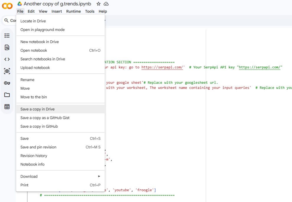
Step 2: Configure your parameters
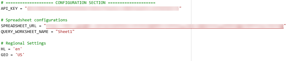
At the top of the script, look for the green section named CONFIGURATION SECTION. This is where you need to update the following variables before running the script:
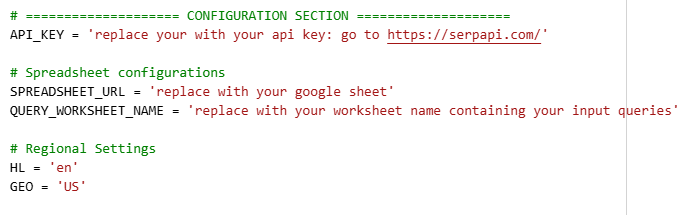
API_KEY
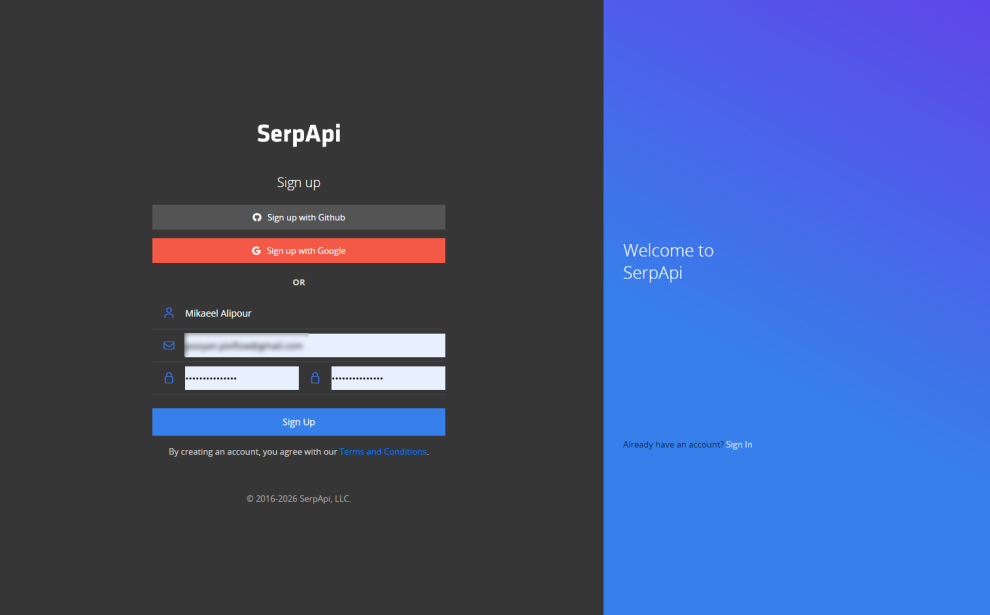
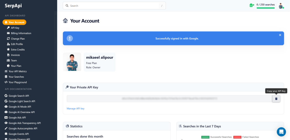
This is what connects your SerpApi account to the script. To get a free API key, sign up at SerpApi and copy your key from your dashboard. Then paste it here.
One thing to plan for: the script runs one API call per keyword, per search property, per timeframe. That’s roughly 45 calls for a single seed keyword.
SerpApi’s free tier (250 searches per month) covers about five seed keywords, which is enough for testing, but a full keyword list will exhaust it quickly. Be sure to check your plan’s monthly limit before you run a large batch.
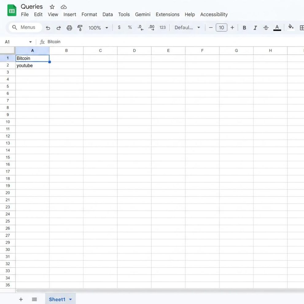
Before you fill in the next fields, create a new Google Sheet and enter your seed keywords in the first column, one per row. These are the terms the script will look up. Start with three to five while you’re testing, so you stay within the free tier. The script reads this column and runs every keyword in it.
SPREADSHEET_URL
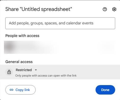
Go to your Google Sheet page and open the sheet where you entered your keywords. This is also where the script will send your data. You don’t need to change any sharing settings.
The script runs under your own Google account, so it can already write to any sheet you own. Just copy the URL from your browser’s address bar and paste it into the script.
QUERY_WORKSHEET_NAME
In the spreadsheet page that contains your seed keywords, at the bottom of the page, you will find a tab. Enter the exact name of the tab (e.g., ‘Sheet1’).
HL
Here you will input your target language code (e.g., ‘en’ for English, ‘fa’ for Farsi).
GEO
This is the section where you will need to input your target country code (e.g., ‘US’ for USA, ‘IR’ for Iran).
Step 3: Run the script
Once your parameters are all set, you are ready to execute the script.
Run each cell by clicking the play icon to its left, or by pressing Ctrl+Enter (Cmd+Enter on Mac). To run everything at once, use Runtime > Run all. Run the cells in sequence from top to bottom.
When prompted, allow the script to authenticate with your Google account so that it can paste the finalized data into your spreadsheet.
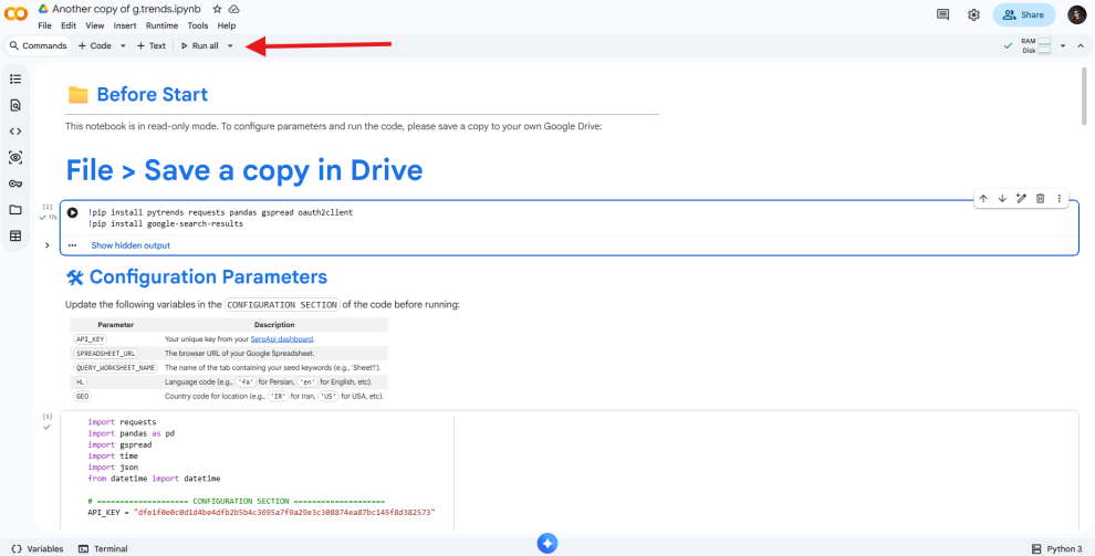
When the script starts running, it will take a few minutes to finish, depending on how many keywords you’re tracking. You can see the progress at the bottom of the script.
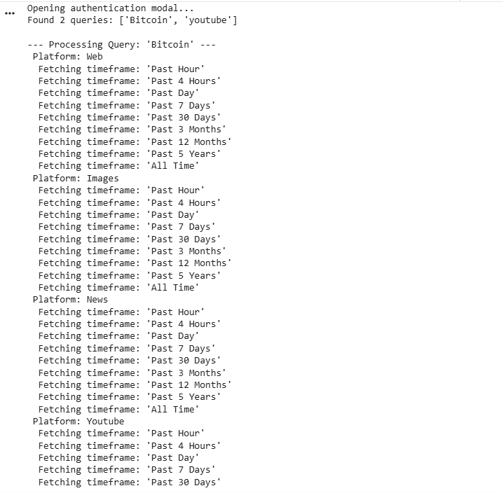
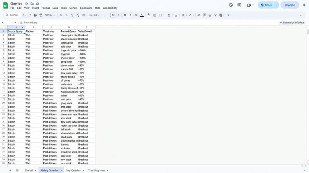
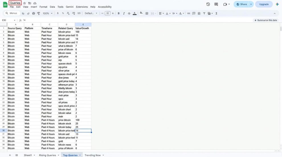
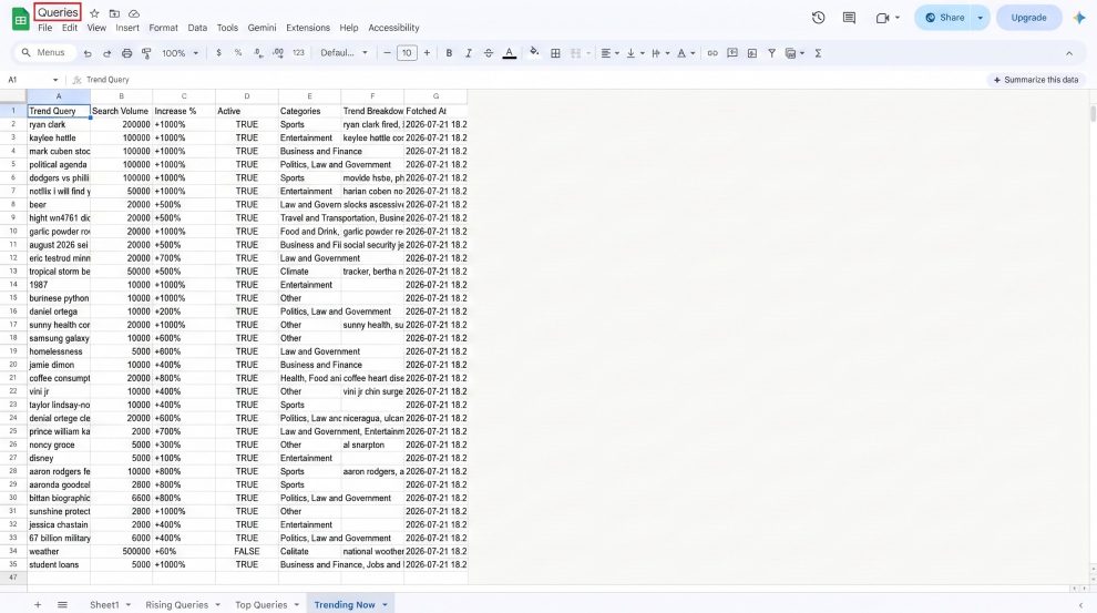
As soon as the process is finished, all the data will be written automatically into new tabs in your Google Sheet.
For the curious: under the hood
If you are wondering exactly how the script processes your keywords, here is a quick look at the logic driving the automation:
- Multi-dimensional looping: The script doesn’t just check standard web search. It uses nested loops to query your seed keywords across five distinct search properties (Web, Images, News, YouTube, and Google Shopping) and nine distinct historical intervals.
- Data parsing: The raw JSON data sent back from SerpApi is massive. The script splits these responses into two clean tables: “rising” queries and “top” queries.
- Understanding the metrics: Historical and related-query data comes from Google’s normalized 0 to 100 interest index, not absolute search volume. A value of 100 denotes peak popularity. However, the script also taps into the Trending Now endpoint, which does provide actual volume bands (e.g., “10K+ searches”) and growth percentages.
Aligning teams and timing the market
Pulling cross-property trends data into a single shared sheet changed how our teams worked together. Previously, SEO, marketing, and social media operated in separate silos, arguing over different dashboards. Having one objective view of consumer interest across the web, YouTube, and news brought everyone to the same table. This made it easy to execute unified, cross-channel campaigns around a single topic.
While social and performance marketing ran short-term promotions, SEO went after the organic search demand. That combined push improved our overall visibility and grew our SEO traffic on those topics, and the other channels saw results too.
The seasonal breakdown also gave us a head start. Standard keyword tools only show monthly averages, so you can’t see when search interest starts to build. By tracking multi-year trends, I could see the week demand started to climb, well before it peaked.
We used that lead time to publish and index content 6 to 8 weeks before the surge hit. By the time competitors noticed the trend in their own tools, our pages were already ranking near the top and picking up the early traffic.
Putting the data to work
Of course, a spreadsheet full of data is only useful if it changes what you do next. Here are the four ways I use these tabs.
Read intent by comparing properties
The script queries every keyword across the different channels: web, images, news, YouTube, and shopping. Comparing those five numbers tells you a lot about what searchers want.
A term climbing on YouTube while web interest stays flat suggests people want a video, so another 2,000-word guide is likely to underperform. A term moving on shopping is transactional and belongs on a product or comparison page. When news is the only property moving, the interest is event-driven and will likely decay within a week or two.
The Google Trends interface can make this comparison, but only one property at a time, which means clicking through and holding numbers in your head. Side by side in a sheet, the pattern takes seconds to read, and it scales to a hundred keywords.
Catch rising queries before your keyword tool does
Traditional keyword tools depend on clickstream data and index refresh cycles, so a genuinely new query can take weeks or months to show a volume figure. Rising queries surface that demand while the volume is still too small to register anywhere else.
Pull rising queries for your head terms weekly, and treat the ones that keep reappearing (not the single-week spikes) as briefs. That’s why it’s worth running the notebook on a schedule rather than ad hoc, so you can compare this week’s rising list with last week’s.
Separate a demand drop from a ranking drop
This one is especially useful when a client asks why their traffic dropped. When traffic to a page falls, pull that keyword’s 12-month interest curve and compare its shape to your Search Console impressions.
If interest fell at the same rate on the same dates, the market moved, and no amount of on-page work will bring it back. If interest held steady while impressions fell, the problem is yours: a ranking loss, an indexing issue, a SERP layout change, a competitor doing something better. Same symptom, two very different next actions, and you can settle it in five minutes instead of a week of auditing.
Time seasonal content to the start of the climb
This is where the longer timeframes help. The short windows show what’s happening now, and the five-year view shows when a topic usually starts to climb. Find the month interest begins to climb, subtract your indexing and ranking lead time (six to eight weeks is a sensible default for anything competitive), and that’s your publish date.
The pattern repeats year over year, so you build the calendar once and reuse it, refreshing the page just before the curve turns up rather than writing from scratch every season.
Key takeaways
By shifting from manual, reactive keyword tracking to a fully programmatic workflow, you can map deep historical interest patterns alongside high-velocity breaking trends in a fraction of the time.
Automating this process with Python, SerpApi, and Google Colab turns messy raw data into one clean sheet your whole team can read. You bypass the traditional headaches of rate-limiting and CAPTCHAs and, instead, build a clean, reliable automation workflow.
I highly encourage you to make a copy of the open-source Colab script, plug in your API key and spreadsheet URL, and experiment with it for your next content planning sprint.